Examples
Important
This page is heavily outdated and under construction. There are many sections that have to be rewritten from ELEKTRONN (legacy) specifics to fit to ELEKTRONN2.
This page gives examples for different use cases of ELEKTRONN2. Besides, the examples are intended to give an idea of how custom network architectures could be created and trained without the built-in pipeline. To understand the examples, basic knowledge of neural networks (e.g. from training) is recommended. The details of the configuration parameters are described here.
A simple 3D CNN
The first example demonstrates how a 3-dimensional CNN and its loss function are specified. The model batch size is 10 and the CNN takes an [23, 183, 183] image volume with 3 channels [1] (e.g. RGB colours) as input.
| [1] | For consistency reasons the axis containing image channels and the axis
containing classification targets are also denoted by 'f' like the
feature maps or features of a MLP. |
Defining the neural network model
The following code snippet [2] exemplifies how a 3-dimensional CNN model can be built using ELEKTRONN2.
| [2] | For complete network config files that you can directly run with little to no modification, see the “examples” directory in the code repository. |
from elektronn2 import neuromancer

image = neuromancer.Input((10, 3, 23, 183, 183), 'b,f,z,x,y', name='image')

# If no node name is given, default names and enumeration are used.
# 3d convolution with 32 filters of size (1,6,6) and max-pool sizes (1,2,2).
conv0 = neuromancer.Conv(image, 32, (1,6,6), (1,2,2))
conv1 = neuromancer.Conv(conv0, 64, (4,6,6), (2,2,2))
conv2 = neuromancer.Conv(conv1, 5, (3,3,3), (1,1,1), activation_func='lin')

# Softmax automatically infers from the input's 'f' axis
# that the number of classes is 5 and the axis index is 1.
class_probs = neuromancer.Softmax(conv2)

# This copies shape and strides from class_probs but the feature axis
# is overridden to 1, the target array has only one feature on this axis,
# the class IDs i.e. 'sparse' labels. It is also possible to use 5
# features where each contains the probability for the corresponding class.
target = neuromancer.Input_like(class_probs, override_f=1, name='target', dtype='int16')

# Voxel-wise loss calculation
voxel_loss = neuromancer.MultinoulliNLL(class_probs, target, target_is_sparse=True)
scalar_loss = neuromancer.AggregateLoss(voxel_loss , name='loss')

# Takes class with largest predicted probability and calculates classification accuracy.
errors = neuromancer.Errors(class_probs, target, target_is_sparse=True)

# Creation of nodes has been tracked and they were associated to a model object.
model = neuromancer.model_manager.getmodel()
model.designate_nodes(input_node=image, target_node=target, loss_node=scalar_loss,
prediction_node=class_probs, prediction_ext=[scalar_loss, errors, class_probs])
model.designate_nodes() triggers printing of aggregated model stats and
extended shape properties of the prediction_node.
Executing the above model creation code prints basic information for each node
and its output shape and saves it to the log file.
Example output:
<Input-Node> 'image'
Out:[(10,b), (3,f), (23,z), (183,x), (183,y)]
---------------------------------------------------------------------------------------
<Conv-Node> 'conv'
#Params=3,488 Comp.Cost=25.2 Giga Ops, Out:[(10,b), (32,f), (23,z), (89,x), (89,y)]
n_f=32, 3d conv, kernel=(1, 6, 6), pool=(1, 2, 2), act='relu',
---------------------------------------------------------------------------------------
<Conv-Node> 'conv1'
#Params=294,976 Comp.Cost=416.2 Giga Ops, Out:[(10,b), (64,f), (10,z), (42,x), (42,y)]
n_f=64, 3d conv, kernel=(4, 6, 6), pool=(2, 2, 2), act='relu',
---------------------------------------------------------------------------------------
<Conv-Node> 'conv2'
#Params=8,645 Comp.Cost=1.1 Giga Ops, Out:[(10,b), (5,f), (8,z), (40,x), (40,y)]
n_f=5, 3d conv, kernel=(3, 3, 3), pool=(1, 1, 1), act='lin',
---------------------------------------------------------------------------------------
<Softmax-Node> 'softmax'
Comp.Cost=640.0 kilo Ops, Out:[(10,b), (5,f), (8,z), (40,x), (40,y)]
---------------------------------------------------------------------------------------
<Input-Node> 'target'
Out:[(10,b), (1,f), (8,z), (40,x), (40,y)]
85
---------------------------------------------------------------------------------------
<MultinoulliNLL-Node> 'nll'
Comp.Cost=640.0 kilo Ops, Out:[(10,b), (1,f), (8,z), (40,x), (40,y)]
Order of sources=['image', 'target'],
---------------------------------------------------------------------------------------
<AggregateLoss-Node> 'loss'
Comp.Cost=128.0 kilo Ops, Out:[(1,f)]
Order of sources=['image', 'target'],
---------------------------------------------------------------------------------------
<_Errors-Node> 'errors'
Comp.Cost=128.0 kilo Ops, Out:[(1,f)]
Order of sources=['image', 'target'],
Prediction properties:
[(10,b), (5,f), (8,z), (40,x), (40,y)]
fov=[9, 27, 27], offsets=[4, 13, 13], strides=[2 4 4], spatial shape=[8, 40, 40]
Total Computational Cost of Model: 442.5 Giga Ops
Total number of trainable parameters: 307,109.
Computational Cost per pixel: 34.6 Mega Ops
The whole model can also be plotted as a graph by using the
elektronn2.utils.d3viz.visualize_model() method:
>>> from elektronn2.utils.d3viz import visualise_model
>>> visualise_model(model, '/tmp/modelgraph')
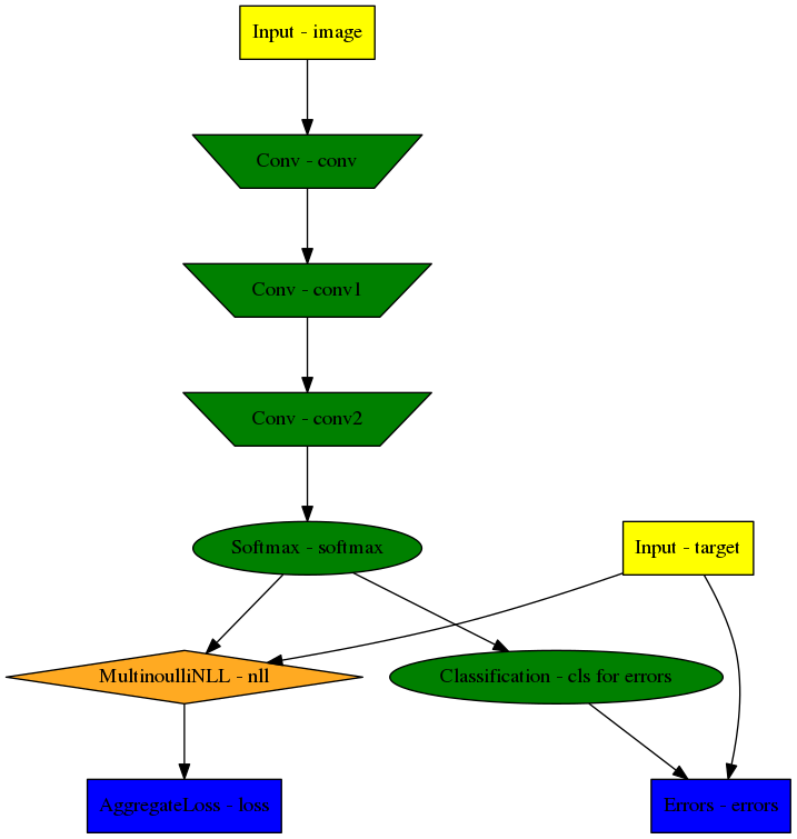
Model graph of the example CNN. Inputs are yellow and outputs are blue.
Some node classes are represented by special shapes, the default shape is oval.
Interactive usage of the Model and Node objects
Node objects can be used like functions to calculate their output.
The first call triggers compilation and caches the compiled function:
>>> test_output = class_probs(test_image)
Compiling softmax, inputs=[image]
Compiling done - in 21.32 s
>>> import numpy as np
>>> np.allclose(test_output, reference_output)
True
The model object has a dict interface to its Nodes:
>>> model
['image', 'conv', 'conv1', 'conv2', 'softmax', 'target', 'nll', 'loss', 'cls for errors', 'errors']
>>> model['nll'] == voxel_loss
True
>>> conv2.shape.ext_repr
'[(10,b), (5,f), (8,z), (40,x), (40,y)]\nfov=[9, 27, 27], offsets=[4, 13, 13],
strides=[2 4 4], spatial shape=[8, 40, 40]'
>>> target.measure_exectime(n_samples=5, n_warmup=4)
Compiling target, inputs=[target]
Compiling done - in 0.65 s
86
target samples in ms:
[ 0.019 0.019 0.019 0.019 0.019]
target: median execution time: 0.01903 ms
For efficient dense prediction, batch size is changed to 1 and MFP is inserted.
To do that, the model must be rebuilt/reloaded.
MFP needs a different patch size. The closest possible one is selected:
>>> model_prediction = neuromancer.model.rebuild_model(model, imposed_batch_size=1,
                                                       override_mfp_to_active=True)
patch_size (23) changed to (22) (size not possible)
patch_size (183) changed to (182) (size not possible)
patch_size (183) changed to (182) (size not possible)
---------------------------------------------------------------------------------------
<Input-Node> 'image'
Out:[(1,b), (3,f), (22,z), (182,x), (182,y)]
...
Dense prediction: test_image can have any spatial shape as long as it
is larger than the model patch size:
>>> model_prediction.predict_dense(test_image, pad_raw=True)
Compiling softmax, inputs=[image]
Compiling done - in 27.63 s
Predicting img (3, 58, 326, 326) in 16 Blocks: (4, 2, 2)
...
Plotting the model graph:
>>> utils.d3viz.visualise_model(model, '/tmp/model')
3D Neuro Data
Important
This section is out of date and has to be revised for ELEKTRONN2
This task is about detecting neuron cell boundaries in 3D electron microscopy image volumes. The more general goal is to find a volume segmentation by assigning each voxel a cell ID. Predicting boundaries is a surrogate target for which a CNN can be trained (see also the note about target formulation here) - the actual segmentation would be made by e.g. running a watershed on the predicted boundary map. This is a typical img-img task.
For demonstration purpose, a very small CNN with only 70k parameters and 5 layers is used. This trains fast but is obviously limited in accuracy. To solve this task well, more training data would be required in addition.
The full configuration file can be found in ELEKTRONN2’s examples folder
as neuro_3d_config.py. Here only selected settings will be mentioned.
Getting Started
Important
This section is out of date and has to be revised for ELEKTRONN2
Download example training data (~100MB):
wget http://elektronn.org/downloads/neuro_data.zip
unzip neuro_data.zip
Edit
save_path, data_path, label_path, preview_data_pathin the config fileneuro_3d_config.pyin ELEKTRONN2’sexamplesfolderRun:
elektronn2-train </path/to_config_file> [ --gpu={Auto|False|<int>}]
Inspect the printed output and the plots in the save directory
Data Set
Important
This section is out of date and has to be revised for ELEKTRONN2
This data set is a subset of the zebra finch area X dataset j0126 by
Jörgen Kornfeld.
There are 3 volumes which contain “barrier” labels (union of cell boundaries
and extra cellular space) of shape (150,150,150) in (x,y,z) axis
order. Correspondingly, there are 3 volumes which contain raw electron
microscopy images. Because a CNN can only make predictions within some offset
from the input image extent, the size of the image cubes is larger
(350,350,250) in order to be able to make predictions (and to train!)
for every labelled voxel. The margin in this examples allows to make
predictions for the labelled region with a maximal field of view of
201 in x,y and 101 in z.
There is a difference in the lateral dimensions and in z - direction
because this data set is anisotropic: lateral voxels have a spacing of
\(10 \mu m\) in contrast to \(20 \mu m\) vertically. Snapshots
of images and labels are depicted below.
During training, the pipeline cuts image and target patches from the loaded data cubes at randomly sampled locations and feeds them to the CNN. Therefore the CNN input size should be smaller than the size of the cubes, to leave enough space to cut from many different positions. Otherwise it will always use the same patch (more or less) and soon over-fit to that one.
Note
Implementation details: When the cubes are read into the pipeline, it
is implicitly assumed that the smaller label cube is spatially centered
w.r.t the larger image cube (hence the size surplus of the image cube must
be even). Furthermore, the cubes are for performance reasons internally
axis swapped to (z, (ch,) x, y) order, zero-padded to the same size and
cropped such that only the area in which labels and images are both
available after considering the CNN offset. If labels cannot be effectively
used for training (because either the image surplus is too small or your FOV
is too large) a note will be printed.
Additionally to the 3 pairs of images and labels, 2 small image cubes for live
previews are included. Note that preview data must be a list of one or
several cubes stored in a h5-file.
CNN design
Important
This section is out of date and has to be revised for ELEKTRONN2
The architecture of the CNN is determined by:
n_dim = 3
filters = [[4,4,1],[3,3,1],[3,3,3],[3,3,3],[2,2,1]]
pool    = [[2,2,1],[2,2,1],[1,1,1],[1,1,1],[1,1,1]]
nof_filters = [10,20,40,40,40]
desired_input = [127,127,7]
batch_size = 1
- Because the data is anisotropic the lateral FOV is chosen to be larger. This reduces the computational complexity compared to a naive isotropic CNN. Even for genuinely isotropic data this might be a useful strategy, if it is plausible that seeing a large lateral context is sufficient to solve the task.
- As an extreme, the presented CNN is partially actually 2D: in the first two
and in the last layer the filter kernels have extent
1inz. Only two middle layers perform a truly 3D aggregation of the features along the third axis. - The resulting FOV is
[31,31,7](to solve this task well, more than100lateral FOV is beneficial...) - Using this input size gives an output shape of
[25,25,3]i.e. 1875 prediction neurons. For training, this is a good compromise between computational cost and sufficiently many prediction neurons to average the gradient over. Too few output pixel result in so noisy gradients that convergence might be impossible. For making predictions, it is more efficient to re-created the CNN with a larger input size (see here). - If there are several
100-1000output neurons, a batch size of1is commonly sufficient and is not necessary to compute an average gradient over several images. - The output shape has strides of
[4,4,1]due to 2 times lateral pooling by 2. This means that the predicted[25,25,3]voxels do not lie laterally adjacent, if projected back to the space of the input image: for every lateral output voxel there are3voxel separating it from the next output voxel - for those no prediction is available. To obtain dense predictions (e.g. when making the live previews) the methodelektronn2.net.convnet.MixedConvNN.predictDense()is used, which moves along the missing locations and stitches the results. For making large scale predictions after training, this can be done more efficiently using MFP (see here). - To solve this task well, about twice the number of layers, several million parameters and more training data are needed.
Training Data Options
Important
This section is out of date and has to be revised for ELEKTRONN2
Config:
valid_cubes = [2,]
grey_augment_channels = [0]
flip_data = True
anisotropic_data = True
warp_on = 0.7
- Of the three training data cubes the last one is used as validation data.
- The input images are grey-valued i.e. they have only 1 channel. For this channel “grey value augmentaion” (randomised histogram distortions) are applied when sampling batches during training. This helps to achieve invariance against varying contrast and brightness gradients.
- During patch cutting the axes are flipped and transposed as a means of data augmentation.
- If the data is anisotropic, the pipeline assumes that the singled-out axis is
z. For anisotropic data axes are not transposed in a way that axes of different resolution get mixed up. - For 70% of the batches the image and labels are randomly warped.
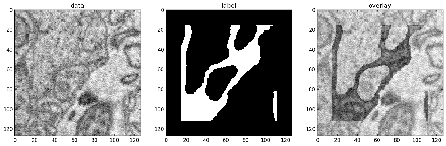
Left: The input data.
Centre: The labels, note the offset.
Right: Overlay of data with labels, here you can check whether they are
properly registered.
During training initialisation a debug plot of a randomly sampled batch is made
to check whether the training data is presented to the CNN in the intended way
and to find errors (e.g. image and label cubes are not matching or labels are
shifted w.r.t to images). Once the training loop has started, more such plots
can be made from the ELEKTRONN2 command line (ctrl+c)
>>> mfk@ELEKTRONN2: self.debugGetCNNBatch()
Note
Training with 2D images:
The shown setup works likewise for training a 2D CNN on this task. Just the
CNN configuration parameters must be adjusted.
Then 2D training patches are cut from the cubes. If
anisotropic_data = True these are cut only from the x,y-plane;
otherwise transposed, too.
Therefore, this setup can be used for actual 2D images if they are stacked to
form a cube along a new “z“-axis. If the 2D images have different shapes
they cannot be stacked but, the 2D arrays can be augmented with a third
dummy-axis to be of shape (x,y,1) and each put in a separate h5-file,
which is slightly more intricate.
Results & Comments
Important
This section is out of date and has to be revised for ELEKTRONN2
- When running this example, commonly the NLL-loss stagnates for about
15kiterations around0.7. After that you should observe a clear decrease. On a desktop with a high-end GPU, with latest theano and cuDNN versions and using background processes for the batch creation the training should runat 15-20 it/s. - Because of the (too) small training data size the validation error should stagnate soon and even go up later.
- Because the model has too few parameters, predictions are typically not smooth and exhibit grating-like patterns - using a more complex model mitigates this effect.
- Because the model has a small FOV (which for this task should rather be increase by more layers than more maxpooling) predictions contain a lot of “clutter” within wide cell bodies: there the CNN does not see the the cell outline which is apparently an important clue to solve this task.
MNIST Examples
Important
This section is out of date and has to be revised for ELEKTRONN2
MNIST is a benchmark data set for handwritten digit recognition/classification. State of the art benchmarks for comparison can be found here.
Note
The data will be automatically downloaded but can also be downloaded manually from here.
CNN with built-in Pipeline
Important
This section is out of date and has to be revised for ELEKTRONN2
In ELEKTRONN2’s examples folder is a file MNIST_CNN_warp_config.py. This
is a configuration for img-scalar training and it uses a different data class
than the “big” pipeline for neuro data. When using an alternative data pipeline,
the options for data loading and batch creation are given given by keyword
argument dictionaries in the Data Alternative section of the config file:
data_class_name      = 'MNISTData'
data_load_kwargs     = dict(path=None, convert2image=True, warp_on=True, shift_augment=True)
data_batch_kwargs    = dict()
This configuration results in:
- Initialising a data class adapted for MNIST from
elektronn2.data.traindata - Downloading the MNIST data automatically if path is
None(otherwise the given path is used) - Reshaping the “flat” training examples (they are stored as vectors of length
784) to
28 x 28matrices i.e. images - Data augmentation through warping (see warping): for each batch in a training iteration random deformation parameters are sampled and the corresponding transformations are applied to the images in a background process.
- Data augmentation through translation:
shift_augmentcrops the28 x 28images to26 x 26(you may notice this in the printed output). The cropping leaves choice of the origin (like applying small translations), in this example the data set size is inflated by factor4. - For the function
getbatchno additional kwargs are required (the warping and so on was specified already with the initialisation).
The architecture of the NN is determined by:
n_dim           = 2           # MNIST are 2D images
desired_input   = 26
filters         = [3,3]       # two conv layers with each 3x3 filters
pool            = [2,2]       # for each conv layer maxpooling by 2x2
nof_filters     = [16,32]     # number of feature maps per layer
MLP_layers       = [300,300]  # numbers of filters for perceptron layers (after conv layers)
This is 2D CNN with two conv layers and two fully connected layers each with 300 neurons. As MNIST has 10 classes, an output layer with 10 neurons is automatically added, and not specified here.
To run the example, make a copy of the config file and adjust the paths. Then
run the elektronn2-train script, and pass the path of your config file:
elektronn2-train </path/to_config_file> [ --gpu={Auto|False|<int>}]
The output should read like this:
Reading config-file ../elektronn2/examples/MNIST_CNN_warp_config.py
WARNING: Receptive Fields are not centered with even field of view (10)
WARNING: Receptive Fields are not centered with even field of view (10)
Selected patch-size for CNN input: Input: [26, 26]
Layer/Fragment sizes:        [[12, 5], [12, 5]]
Unpooled Layer sizes:        [[24, 10], [24, 10]]
Receptive fields:    [[4, 10], [4, 10]]
Strides:             [[2, 4], [2, 4]]
Overlap:             [[2, 6], [2, 6]]
Offset:              [5.0, 5.0].
If offset is non-int: output neurons lie centered on input neurons,they have an odd FOV

Overwriting existing save directory: /home/mfk/CNN_Training/2D/MNIST_example_warp/
Using gpu device 0: GeForce GTX TITAN
Load ELEKTRONN2 Core
10-class Data Set: #training examples: 200000 and #validing: 10000
MNIST data is converted/augmented to shape (1, 26, 26)
------------------------------------------------------------
Input shape   =  (50, 1, 26, 26) ; This is a 2 dimensional NN
---
2DConv: input= (50, 1, 26, 26)       filter= (16, 1, 3, 3)
Output = (50, 16, 12, 12) Dropout OFF, Act: relu pool: max
Computational Cost: 4.1 Mega Ops
---
2DConv: input= (50, 16, 12, 12)      filter= (32, 16, 3, 3)
Output = (50, 32, 5, 5) Dropout OFF, Act: relu pool: max
Computational Cost: 23.0 Mega Ops
---
PerceptronLayer( #Inputs = 800 #Outputs = 300 )
Computational Cost: 12.0 Mega Ops
---
PerceptronLayer( #Inputs = 300 #Outputs = 300 )
Computational Cost: 4.5 Mega Ops
---
PerceptronLayer( #Inputs = 300 #Outputs = 10 )
Computational Cost: 150.0 kilo Ops
---
GLOBAL
Computational Cost: 43.8 Mega Ops
Total Count of trainable Parameters: 338410
Building Computational Graph took 0.030 s
Compiling output functions for nll target:
    using no class_weights
    using no example_weights
    using no lazy_labels
    label propagation inactive
A few comments on the expected output before training:
- There will be a warning that receptive fields are not centered (the neurons in the last conv layer lie spatially “between” the neurons of the input layer). This is ok because this training task does require localisation of objects. All local information is discarded anyway when the fully connected layers are put after the conv layers.
- The information of
elektronn2.net.netutils.CNNCalculator()is printed first, i.e. the layer sizes, receptive fields etc. - Although MNIST contains only 50000 training examples, it will print 200000 because of the shift augmentation, which is done when loading the data
- For image training, an auxiliary dimension for the (colour) channel is introduced.
- The input shape
(50, 1, 26, 26)indicates that the batch size is 50, the number of channels is just 1 and the image extent is26 x 26. - You can observe that the first layer outputs an image of size is
12 x 12: the convolution with filter size 3 reduces 26 to 24, then the maxpooling by factor 2 reduces 24 to 12. - After the last conv layer everything except the batch dimension is flattened
to be feed into a fully connected layer:
32 x 5 x 5 == 800. If the image extent is not sufficiently small before doing this (e.g.10 x 10 == 100) this will be a bottleneck and introduce huge weight matrices for the fully connected layer; more poolings must be used then.
Results & Comments
Important
This section is out of date and has to be revised for ELEKTRONN2
The values in the example file should give a good result after about 10-15 minutes on a recent GPU, but you are invited to play around with the network architecture and meta-parameters such as the learning rate. To watch the progress (in a nicer way than the reading the printed numbers on the console) go to the save directory and have a look at the plots. Every time a new line is printed in the console, the plot gets updated as well.
If you had not used warping the progress of the training would look like this:
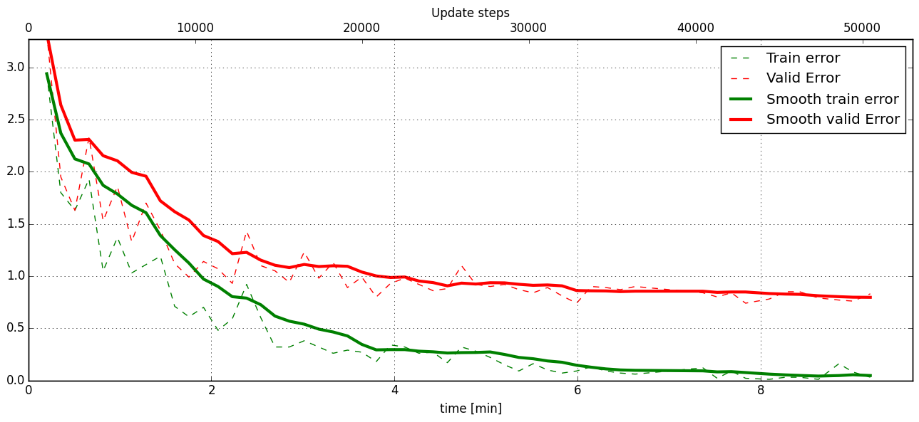
Withing a few minutes the training error goes to 0 whereas the validation error stays on a higher level.
The spread between training and validation set (a partition of the data not presented as training examples) indicates a kind of over-fitting. But actually the over-fitting observed here is not as bad as it could be: because the training error is 0 the gradients are close to 0 - no weight updates are made for 0 gradient, so the training stops “automatically” at this point. For different data sets the training error might not reach 0 and weight updates are made all the time resulting in a validation error that goes up after some time - this would be real over-fitting.
A common regularisation technique to prevent over-fitting is drop out which is also implemented in ELEKETRONN. But since MNIST data are images, we want to demonstrate the use of warping instead in this example.
Warping makes the training goal more difficult, therefore the CNN has to learn its task “more thoroughly”. This greatly reduces the spread between training and validation set. Training also takes slightly more time. And because the task is more difficult the training error will not reach 0 anymore. The validation error is also high during training, since the CNN is devoting resources to solving the difficult (warped) training set at the expense of generalization to “normal” data of the validation set.
The actual boost in (validation) performance comes when the warping is turned
off and the training is fine-tuned with a smaller learning rate. Wait until the
validation error approximately plateaus, then interrupt the training using
Ctrl+c:
>>> data.warp_on = False # Turn off warping
>>> setlr 0.002          # Lower learning rate
>>> q                    # quit console to continue training
This stops the warping for further training and lowers the learning rate. The resulting training progress would look like this:
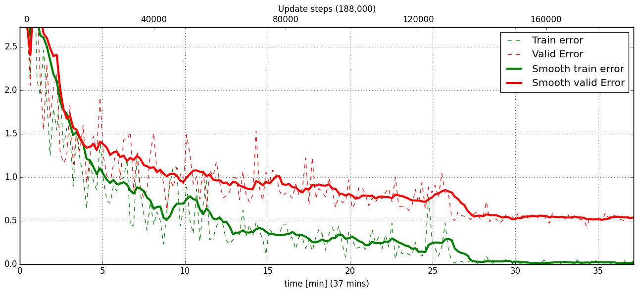
The training was interrupted after ca. 130000 iterations. Turning off warping reduced both errors to their final level (after the gradient is 0 again, no progress can be made).
Because our decisions on the best learning rate and the best point to stop warping have been influenced by the validation set (we could somehow over-fit to the validation set), the actual performance is evaluated on a separate, third set, the test set (we should really only ever look at the test error when we have decided on a training setup/schedule, the test set is not meant to influence training at all).
Stop the training using ctrl+c:
>>> print self.testModel('test')
(<NLL>, <Errors>)
The result should be competitive - around 0.5% error, i.e. 99.5% accuracy.
MLP with built-in Pipeline
Important
This section is out of date and has to be revised for ELEKTRONN2
In the spirit of the above example, MNIST can also be trained with a pure multi
layer perceptron (MLP) without convolutions. The images are then just flattened
vectors (–> vect-scalar mode). There is a config file MNIST_MLP_config.py
in the Examples folder. This method can also be applied for any other
non-image data, e.g. predicting income from demographic features.
Standalone CNN
Important
This section is out of date and has to be revised for ELEKTRONN2
If you think the big pipeline and long configuration file is a bit of an
overkill for good old MNIST we have an alternative lightweight example in the
file MNIST_CNN_standalone.py of the Examples folder. This example
illustrates what (in a slightly more elaborate way) happens under the hood of
the big pipeline.
First we import the required classes and initialise a training data object from
elektronn2.training.traindata (which we actually used above, too). It
does not more than loading the training, validation and testing data and sample
batches randomly - all further options e.g. for augmentation are not used here:
from elektronn2.training.traindata import MNISTData
from elektronn2.net.convnet import MixedConvNN

data = MNISTData(path='~/devel/ELEKTRONN2/Examples/mnist.pkl',convert2image=True, shift_augment=False)
Next we set up the Neural Network. Each method of cnn has much more options
which are explained in the API doc. Start with similar code if you want to
create customised NNs:
batch_size = 100
cnn = MixedConvNN((28,28),input_depth=1) # input_depth: only 1 gray channel (no RGB or depth)
cnn.addConvLayer(10,5, pool_shape=2, activation_func="abs") # (nof, filtersize)
cnn.addConvLayer(8, 5, pool_shape=2, activation_func="abs")
cnn.addPerceptronLayer(100, activation_func="abs")
cnn.addPerceptronLayer(80, activation_func="abs")
cnn.addPerceptronLayer(10, activation_func="abs") # need 10 outputs as there are 10 classes in the data set
cnn.compileOutputFunctions()
cnn.setOptimizerParams(SGD={'LR': 1e-2, 'momentum': 0.9}, weight_decay=0) # LR: learning rate
Finally, the training loop which applies weight updates in every iteration:
for i in range(5000):
    d, l = data.getbatch(batch_size)
    loss, loss_instance, time_per_step = cnn.trainingStep(d, l, mode="SGD")

    if i%100==0:
        valid_loss, valid_error, valid_predictions = cnn.get_error(data.valid_d, data.valid_l)
        print("update:",i,"; Validation loss:",valid_loss, "Validation error:",valid_error*100.,"%")

loss, error, test_predictions = cnn.get_error(data.test_d, data.test_l)
print "Test loss:",loss, "Test error:",error*100.,"%"
Of course the performance of this setup is not as good of the model above, but
feel free tweak - how about dropout? Simply add enable_dropout=True to the
cnn initialisation: all layers have by default a dropout rate of 0.5 - unless it
is suppressed with force_no_dropout=True when adding a particular layer (it
should not be used in the last layer). Don’t forget to set the dropout rates to
0 while estimating the performance and to their old value afterwards (the
methods cnn.getDropoutRates and cnn.setDropoutRates might be useful).
Hint: for dropout, a different activation function than abs, more neurons
per layer and more training iterations might perform better... you can try
adapting it yourself or find a ready setup with drop out in the examples
folder.
Auto encoder Example
Important
This section is out of date and has to be revised for ELEKTRONN2
This examples also uses MNIST data, but this time the task is not classification
but compression. The input images have shape 28 x 28 but we will regard them
as 784 dimensional vectors. The NN is shaped like an hourglass: the number of
neurons decreases from 784 input neurons to 50 internal neurons in the central
layer. Then the number increases symmetrically to 784 for the output. The
training target is to reproduce the input in the output layer (i.e. the labels
are identical to the data). Because the inputs are float numbers, so is the
output and this is a regression problem. The first part of the auto encoder
compresses the information and the second part decompresses it. The weights of
both parts are shared, i.e. the weight matrix of each decompression layer is the
transposed weight matrix of the corresponding compression layer, and updates are
made simultaneously in both layers. For constructing an auto encoder the method
cnn.addTiedAutoencoderChain is used.
import matplotlib.pyplot as plt

from elektronn2.training.traindata import MNISTData
from elektronn2.net.convnet import MixedConvNN
from elektronn2.net.introspection import embedMatricesInGray


# Load Data #
data = MNISTData(path='/docs/devel/ELEKTRONN2/elektronn2/examples/mnist.pkl',convert2image=False, shift_augment=False)


# Load Data #
data = MNISTData(path='~/devel/ELEKTRONN2/Examples/mnist.pkl',convert2image=False, shift_augment=False)

# Create Autoencoder #
batch_size = 100
cnn = MixedConvNN((28**2),input_depth=None)
cnn.addPerceptronLayer( n_outputs = 300, activation_func="tanh")
cnn.addPerceptronLayer( n_outputs = 200, activation_func="tanh")
cnn.addPerceptronLayer( n_outputs = 50, activation_func="tanh")
cnn.addTiedAutoencoderChain(n_layers=None, activation_func="tanh",input_noise=0.3, add_layers_to_network=True)
cnn.compileOutputFunctions(target="regression")  #compiles the cnn.get_error function as well
cnn.setOptimizerParams(SGD={'LR': 5e-1, 'momentum': 0.9}, weight_decay=0)

for i in range(10000):
    d, l = data.getbatch(batch_size)
    loss, loss_instance, time_per_step = cnn.trainingStep(d, d, mode="SGD")

    if i%100==0:
        print("update:",i,"; Training error:", loss)

loss,  test_predictions = cnn.get_error(data.valid_d, data.valid_d)

plt.figure(figsize=(14,6))
plt.subplot(121)
images = embedMatricesInGray(data.valid_d[:200].reshape((200,28,28)),1)
plt.imshow(images, interpolation='none', cmap='gray')
plt.title('Data')
plt.subplot(122)
recon = embedMatricesInGray(test_predictions[:200].reshape((200,28,28)),1)
plt.imshow(recon, interpolation='none', cmap='gray')
plt.title('Reconstruction')

cnn.saveParameters('AE-pretraining.param')
The above NN learns to compress the 784 pixels of an image to a 50 dimensional code (ca. 15x). The quality of the reconstruction can be inspected from plotting the images and comparing them to the original input:
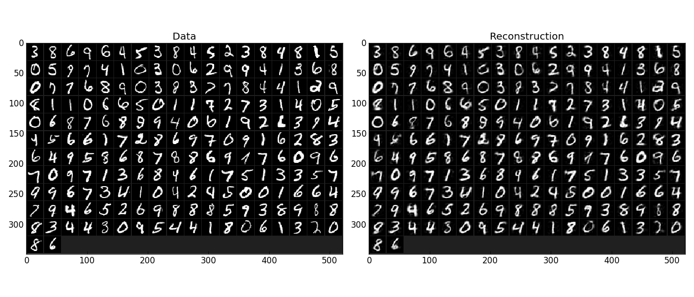
Left input data (from validation set) and right reconstruction. The reconstruction values have been slightly rescaled for better visualisation.
The compression part of the auto encoder can be used to reduce the dimension of a data vector, while still preserving the information necessary to reconstruct the original data.
Often training data (e.g. lots of images of digits) are vastly available but nobody has taken the effort to create training labels for all of them. This is when auto encoders can be useful: train an auto encoder on the unlabelled data and use the learnt weights to initialise a NN for classification (aka pre-training).The classifcation NN does not have to learn a good internal data representation from scratch. To fine-tune the weights for classification (mainly in the additional output layer), only a small fraction of the examples must be labelled. To construct a pre-trained NN:
cnn.saveParameters('AE-pretraining.param', layers=cnn.layers[0:3]) # save the parameters for the compression part
cnn2 = MixedConvNN((28**2),input_depth=None) # Create a new NN
cnn2.addPerceptronLayer( n_outputs = 300, activation_func="tanh")
cnn2.addPerceptronLayer( n_outputs = 200, activation_func="tanh")
cnn2.addPerceptronLayer( n_outputs = 50, activation_func="tanh")
cnn2.addPerceptronLayer( n_outputs = 10, activation_func="tanh") # Add a layer for 10-class classificaion
cnn2.compileOutputFunctions(target="nll")  #compiles the cnn.get_error function as well # target function nll for classification
cnn2.setOptimizerParams(SGD={'LR': 0.005, 'momentum': 0.9}, weight_decay=0)
cnn2.loadParameters('AE-pretraining.param') # This overloads only the first 3 layers,because the file contains only params for 3 layers

# Do training steps with the labels like
for i in range(10000):
    d, l = data.getbatch(batch_size)
    cnn2.trainingStep(d, l, mode="SGD")
RNN Example
Note
Coming soon